

What I learned building search for a camera shop
How do we help someone find the right camera? A practical look at full-text, vector and hybrid search, how their indexes stay current, and the trade-offs behind a useful search system.
Search is an indispensable part of many modern retail applications. Take an online camera shop, for instance. It could have exactly what you need, but if you can’t find it, you might as well shop somewhere else.
Imagine we’re building that shop, with a few thousand cameras, lenses and accessories. Some customers know exactly what they want, say a “Sony ZV-E10” (my camera). Others can only describe a need: “a compact camera for filming myself”. One request asks for a particular model; the other needs us to connect an activity to suitable products.
A vector database might seem like a natural way to handle these different kinds of requests. It can find related product descriptions even when the words differ. But if I ask for a Sony ZV-E10, another Sony vlogging camera is still the wrong model.
In this article, we’ll explore full-text, vector and hybrid search using a camera-shop demo I built for a talk. It uses Redis, but the design questions apply more generally. We’ll start with matching words and work towards combining the methods. Along the way, we’ll ask what happens when a new camera hasn’t reached search yet, how to replace an index while customers keep searching, and how much time better results can cost.
What do we know about a product?
Before choosing how to search, let’s look at what we have. The demo contains 2,317 products from photography-related queries in Amazon’s ESCI dataset. Here is the ZV-E10 record, with two excerpts from its bullet points:
| Field | Value |
|---|---|
product_id | B09BBKVMCD |
product_title | Sony Alpha ZV-E10 - APS-C Interchangeable Lens Mirrorless Vlog Camera - White |
product_description | null |
product_bullet_point | “Large 24.2MP APS-C Exmor CMOS Sensor and fast BIONZ X processor”; “Easy live streaming w/ single USB cable and no extra hardware/software” |
product_brand | Sony |
product_color | White |
product_locale | us |
The title helps identify the model. The bullet points describe capabilities. Brand and colour can become filters. The description is missing, so we’ll work with the text we have.
Before we try searching that text, we should decide what would count as a useful result. If you search for Sony ZV-E10, you probably want the camera body or a kit containing it. For this example, that’s what we’ll count as a match. A strap that fits the camera won’t count, however often its description mentions the model.
Start with the words in the query
Let’s start with the customer who knows the model they want. A straightforward first attempt would be to check whether a product title contains their query. We have the titles and we have the query, so we can compare the strings.
It doesn’t take much thinking to see where this breaks. Someone searching for sony zv e10 won’t literally match Sony ZV-E10. Lowercasing takes care of the capitals, but we still have to deal with the punctuation. Another person might type zv e10 sony, or search for a feature that appears only in the bullet points.
We can make this more flexible by breaking the words in the product titles, descriptions and bullet points into searchable terms, a process called tokenisation. We do the same with the query, then look for matching terms. The words no longer have to appear as one continuous string in the same order.
But we’d still have a lot of reading to do if we checked every listing for every query. This is where an inverted index helps. It’s a separate lookup structure that records which searchable documents contain each term, so we can go directly to the matches.
Here, a document simply means a searchable text record. For illustration, let’s use three short listings:
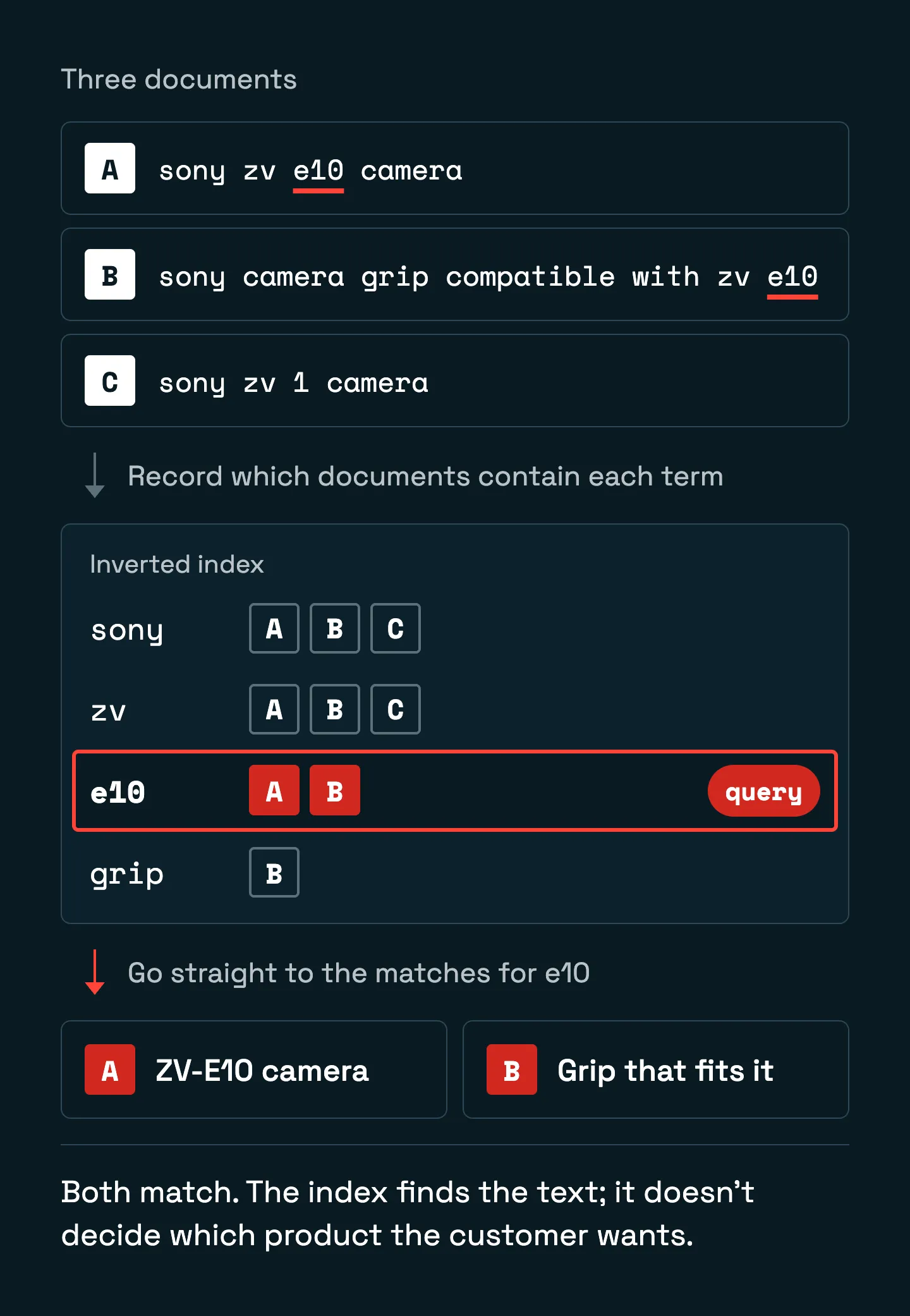
We can now find the listings that contain our search terms. But notice that the camera grip is still there. Its description mentions the ZV-E10 because it fits that camera.
That makes sense from a word-matching perspective. As a customer, though, I would still want the camera to appear first. So we have another problem to solve: how do we decide which matching products should come before the others?
It helps to think about what the words tell us. “Camera” appears throughout our catalogue, so finding it in a listing doesn’t narrow things down very much. A model identifier such as e10 is more distinctive. We would want that term to carry more weight.
Repeated mentions might also be useful evidence, but only up to a point. A description saying “camera” twenty times shouldn’t become twenty times as relevant. And longer descriptions have more opportunities to contain our search terms simply because they have more words.
BM25 combines these ideas into a relevance score. It gives more weight to terms found in fewer documents, using inverse document frequency, or IDF. It considers how often a term appears in a document, with diminishing returns. It also adjusts for document length relative to the collection.
Let’s search our three short listings for sony zv e10. These scores use only those three documents as the collection, rather than the full catalogue:
| Document text | BM25 score |
|---|---|
sony zv e10 camera | 0.80 |
sony camera grip compatible with zv e10 | 0.63 |
sony zv 1 camera | 0.29 |
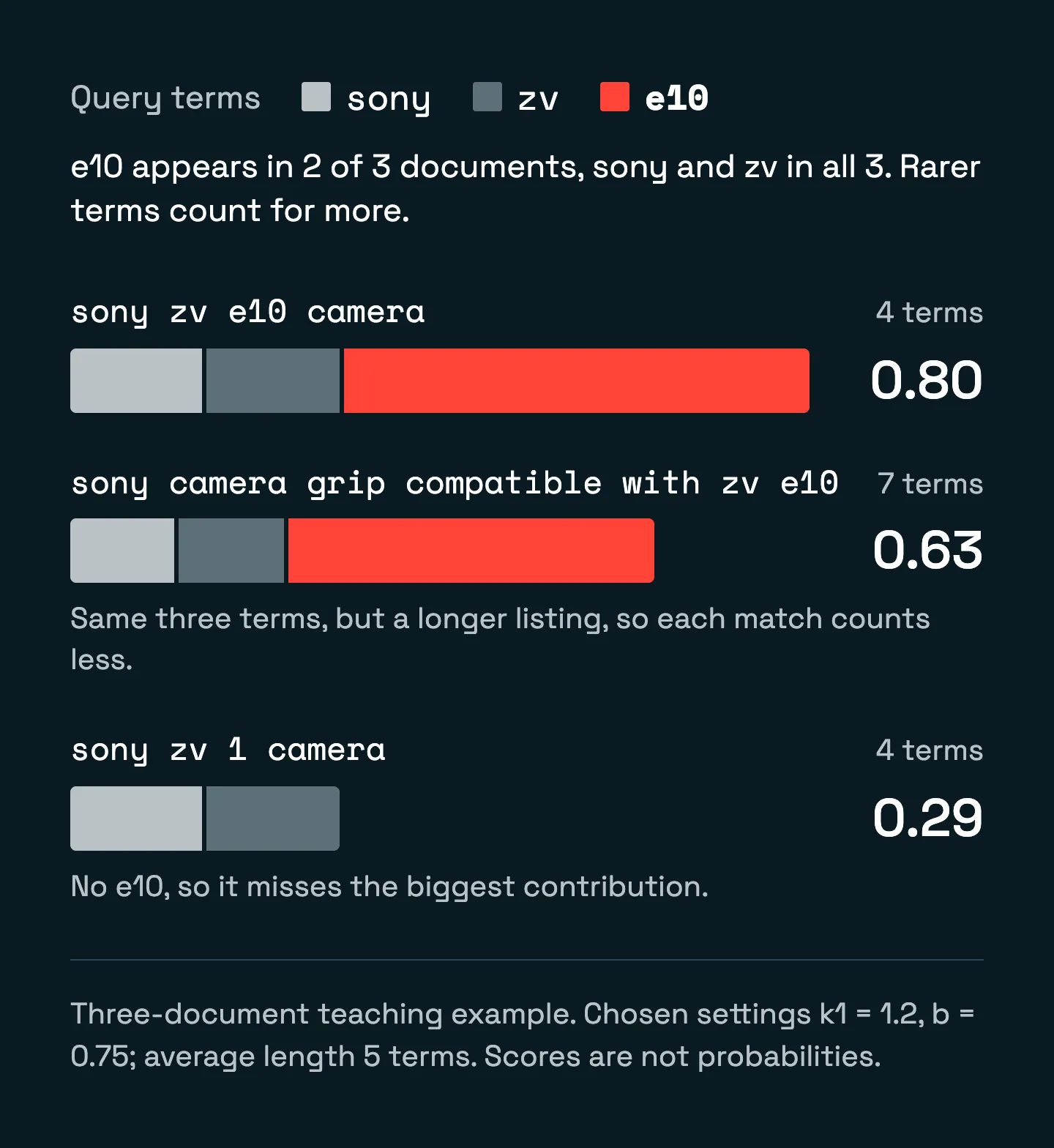
Look at the first two documents. They both contain all three query terms, but the shorter camera listing scores higher because of the length adjustment. The third document lacks e10, the most distinctive query term in this little collection, so it loses that contribution altogether.
This gives us our full-text search baseline, also called lexical search: match the terms, then rank the matching documents. The score doesn’t guarantee that the camera will always beat the grip; changing the descriptions or collection can change the ranking. Nor does 0.80 mean an 80% chance that a product is useful. We still judge usefulness against the customer’s request.
Now let’s apply this approach to the real catalogue. Before we build the index, we need to decide what each searchable document will contain.
Our examples used one short text per product. In the demo, I searched smaller pieces of each listing, called passages. This lets a query match a relevant part of a long listing without treating the whole listing as one document. I took the title, description and bullet-point fields, skipped any empty ones, and split long fields into overlapping chunks.
The ZV-E10 is a simple example: its title becomes one passage and its bullet points become another. It has no description, so there is no description passage. Here are excerpts from the two:
| Passage source | Text (shortened) |
|---|---|
product_title | Sony Alpha ZV-E10 - APS-C Interchangeable Lens Mirrorless Vlog Camera - White |
product_bullet_point | Large 24.2MP APS-C Exmor CMOS Sensor and fast BIONZ X processor … Easy live streaming w/ single USB cable and no extra hardware/software |
Each passage keeps the product ID, the field it came from and its position in that field. To make it searchable, I put a short prefix drawn from the title, brand and colour before the passage text and store the combination as search_text. A passage about USB streaming then carries the camera’s name as well. You can see the complete passage records in the demo. Across the catalogue, our 2,317 products produce 8,472 passages.
Redis stores these passages as JSON records. The demo’s index schema tells Redis how to search them: search_text is a text field for word matching, while product ID, brand and colour are tag fields for exact filtering. We’ll add vector search to this picture shortly.
I use RedisVL, a Python library, to work with that index. Its SearchIndex takes the schema; create() creates the index, and load(..., id_field="passage_id") writes the prepared records for Redis to index. The passage preparation happens in our application. The RedisVL getting-started guide walks through the schema, creation and loading steps.
With those records indexed, a full-text query looks like this. BM25STD is the name of Redis’s standard BM25 scorer:
from redisvl.query import TextQuery

query = TextQuery(
    text="sony zv e10",
    text_field_name="search_text",
    text_scorer="BM25STD",
    num_results=100,
)
Before building the query, the app turns punctuation into spaces, so Sony ZV-E10 becomes Sony ZV E10. This query finds passages containing any of sony, zv or e10, then uses BM25 to rank them.
The query returns passages, so one camera can appear several times. Before displaying the results, the app keeps the first eligible passage for each product and fetches the original product record. Five matching passages won’t necessarily give us five different products. The results can still include the grip, because its listing mentions the model’s name.
For an exact model lookup, we could give each camera a separate model field and store a consistent value such as sony-zv-e10. Then we could look up that value directly. Full-text search remains useful for broader descriptions. For word matching to work, the query and stored text need compatible tokenisation rules, including how they handle punctuation.
What if the customer doesn’t know the right words?
So far, we’ve relied on the customer and the listing using matching terms. Now let’s return to our other request: “a compact camera for filming myself”. A useful result needs evidence for both portability and self-recording.
A product might be described as a “vlogging camera”. We can see the connection between vlogging and filming ourselves, but the words are different. Breaking them into terms more carefully won’t, by itself, give our search system that connection.
This is where embeddings become useful. An embedding model converts text into a vector, which is a list of numbers. Through training, the model learns representations that capture relationships between inputs. For retrieval, we want a query and passages that answer it to end up close to each other under the model’s similarity measure.
Remember the passages we prepared from the product fields? We generate an embedding for each of those ahead of time. When someone searches, we embed their query with the same model and compare it with the stored vectors. The embedding model produces the representations, and the vector index organises the search over them.
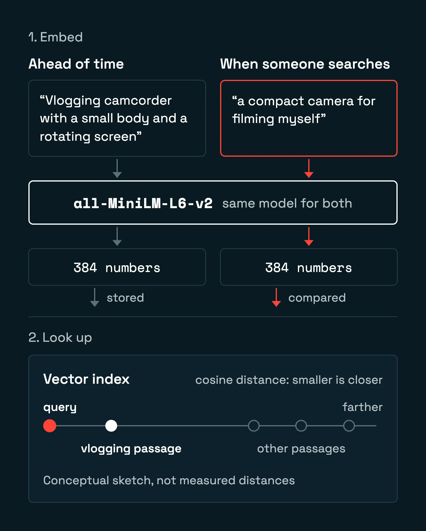
The model in this application is all-MiniLM-L6-v2. It produces 384-dimensional embeddings, so each passage becomes a list of 384 numbers. During preparation, we embed each passage’s search_text and add the resulting list to its JSON record as embedding. The schema declares this as a 384-dimensional vector field using cosine distance. Cosine compares vector directions, and smaller distances returned by Redis mean closer matches.
I’ve written a separate explanation of the dot product and similarity if you’d like to explore the maths behind comparing vectors.
Once we have the query embedding, we can ask for nearby passages:
from redisvl.query import VectorQuery


def search_nearby(query_embedding: list[float]) -> VectorQuery:
    return VectorQuery(
        vector=query_embedding,
        vector_field_name="embedding",
        num_results=100,
    )
For “a compact camera for filming myself”, full-text search returned a video head, which is an accessory. Vector search returned a complete camcorder whose listing describes a small body and a rotating screen. That gave us evidence for the portability and self-recording requirements we’d written down. Here, searching by the learned representation helped us find a more useful kind of product.
Now try the model-name query, sony zv e10. Vector search put a ZV-1 bundle ahead of the ZV-E10 I asked for, which appeared fifth in the product results.
Here, distance measures how close the query and passage embeddings are. It doesn’t count the character edits needed to turn one string into another, as Levenshtein distance does. The model represents the passage’s content, so different wording about the same activity can be close. The cameras’ similar purpose may help explain the result, but it doesn’t make the ZV-1 the model the customer requested.
We have a method that helped with the described activity, but struggled with the specific model. That gives us a reason to keep both kinds of evidence in the search.
Combine what each method knows
One way to use both kinds of evidence is to run lexical and vector retrieval for the same query, then combine their results. That is the demo’s form of hybrid search. We now have two ranked lists and need to turn them into one.
We could try combining the scores, but they need different interpretations. The lexical branch returns a BM25 score, where higher is better. The vector branch returns a cosine distance, where lower is better. Before combining them, we’d need to make their scales comparable and make higher values mean better matches in both.
One option is to convert the cosine distance to a similarity score, normalise the scores from each branch, then take a weighted combination:
combined score = α × normalised lexical score
               + (1 − α) × normalised vector score
Here, α controls how much the lexical score contributes. Normalising the ranges makes combination possible, but it leaves choices about the normalisation method, candidate set and weight.
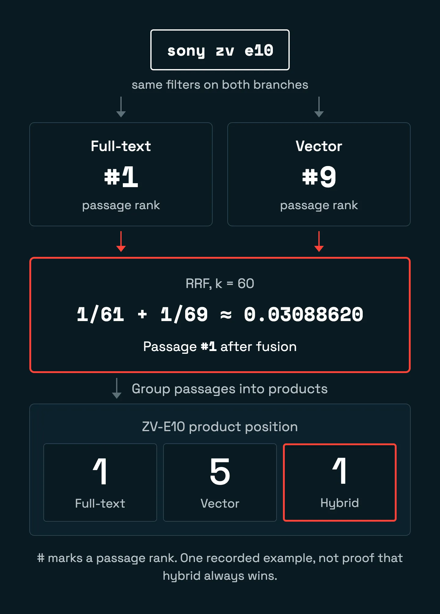
The demo uses another option: the positions in the rankings. We know which passage came first, second and third in each list, even if the score scales differ. Reciprocal rank fusion, or RRF, combines those positions:
RRF score = 1 / (k + lexical rank) + 1 / (k + vector rank)Ranks start at one. As a rank gets larger, its contribution gets smaller. A passage that appears high in both lists gets contributions from both; one missing from a branch’s candidate list gets no contribution from that branch.
The constant k controls how quickly the contributions decrease. A larger value makes neighbouring ranks contribute more similarly. The demo uses k = 60, the value in the original RRF paper, with up to 100 candidate passages from each branch.
Let’s use the ZV-E10 to make this concrete. Its winning passage was first in the lexical ranking and ninth in the vector ranking. Its fused score was therefore 1/61 + 1/69, approximately 0.03088620. That put it first after fusion.
You might remember that the ZV-E10 was fifth in the vector results earlier. That was its product position. Here we’re combining passage rankings, before removing duplicates. Once we turn the passages back into products, the ZV-E10’s positions are full-text 1, vector 5 and hybrid 1.
Try the RRF calculation
Redis runs both branches and combines them through FT.HYBRID. It supports RRF and linear fusion, but I haven’t compared those two approaches in this demo.
Using ranks has a cost, though: we lose how far apart the original scores were. If first place was only slightly ahead of second in one list, and far ahead in another, the ranks alone won’t capture that difference. RRF also can’t recover a passage that neither branch retrieved. We still need our evaluation to tell us whether the combined ranking is useful.
What came back?
We’ve seen how the methods differ on individual queries. Let’s put them alongside each other and return to the question we started with: are we finding useful products?
Before searching, I wrote down what a good answer would be. For a model name, I listed the products I’d accept. For an activity, I listed what the product needed to do. I also used the same filters for each method. Selecting Sony in a brand filter limits results to that brand; typing “Sony camera” gives the search engine words to match.
The demo has ten model-identification cases, covering the Sony ZV-E10, Nikon D610 and Canon RF 85mm F1.2 L USM. They vary the wording and include explicit brand filters. Each lists acceptable product IDs; success means finding at least one among the first three products.
| Retrieval method | Acceptable product in the first three |
|---|---|
| Full-text | 10/10 |
| Vector | 7/10 |
| Hybrid | 10/10 |
Lexical matching did the job for these model requests. Hybrid kept acceptable products in the first three too, but didn’t improve on that success rate. The reason to investigate embeddings comes from the other kind of request, where the customer describes an activity.
For the model requests, we checked whether an acceptable product appeared in the first three results. For these broader requests, let’s look closely at the first result and ask what makes it useful. I tried three queries, including the self-recording example we saw earlier. Here are the first product results, with shortened titles. The judgements below use what the stored listings say about their capabilities:
| Request | Full-text | Vector | Hybrid |
|---|---|---|---|
| Compact camera for filming myself | Manfrotto video head | Vmotal vlogging camcorder | AbergBest digital camera |
| Camera for taking photos underwater | ISHARE waterproof kids camera | Kodak underwater disposable camera | ISHARE waterproof kids camera |
| Lens for photographing distant wildlife | Canon camera-and-lens bundle | Ansee binocular camera | My Animal Command trail camera |
Three things stand out when we look beyond the product names.
Combining the methods can move a useful result down. Vector search put the Vmotal camcorder first for filming ourselves. Hybrid moved it to fifth. The AbergBest camera above it supported compact video capture, but its listing didn’t tell us whether it suited self-recording. Hybrid had helped with the ZV-E10 query; here, it moved the result with clearer supporting information down the list.
A query can leave room for very different good answers. All three underwater results passed our broad check: their listings said they could take photos underwater. Yet a child’s digital camera and a disposable film camera suit different customers. Asking how deep someone plans to go, or whether they want digital photos, would help us choose between them. Changing the ranking can’t supply those missing preferences.
A related product can still be the wrong thing to sell. We asked for a wildlife lens. The first results were a camera bundle, binoculars with a camera, and a trail camera. None passed the lens-only check. Full-text search did have a Tamron 70–300mm lens in fourth place, so at least one lens was making it into the results. We still need to distinguish lenses from complete cameras, then ask which camera the lens must fit.
These results point to different next steps: check what fusion promotes, ask for missing preferences, and add reliable product-type and lens-mount fields. Brand and colour alone can’t express all the constraints a shopper cares about. This is what makes evaluation useful: the results tell us which part of the shop needs work.
Three examples don’t establish a general winner. The activity results and review notes retain the checks and returned products so we can repeat the comparison. For a real shop, we’d add misspellings, accessory requests and things we don’t sell, then keep some judged queries aside to test changes on examples we haven’t tuned against.
Keeping search current
The wildlife results give us a reason to improve our product information. We also need those changes to become searchable. In a working shop, that’s a continuing job: products get added, descriptions change, and listings disappear while customers are searching.
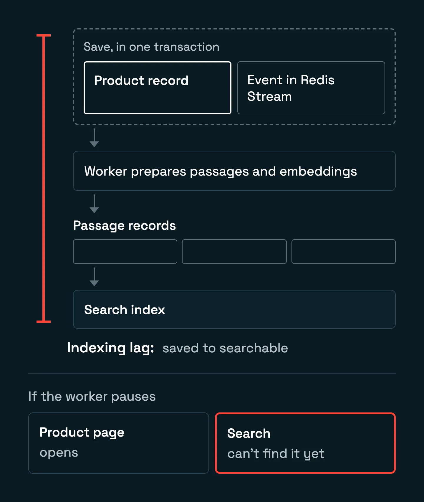
Suppose we add a new camera. Its product page opens correctly, but searching for its name returns nothing. We now have three layers to keep in step:
Source product records → derived passage records → search indexes over those passages.
All three can live inside Redis, but they have different jobs. Saving a product doesn’t, by itself, prepare its passages and embeddings. The index is a separate structure built over those prepared records.
In the demo, that preparation happens in the background. The app saves the product and records the change in a Redis Stream, a log of events that workers can read and process. A worker picks it up, prepares the passages and writes them for Redis to index. Pausing that worker lets us see the gap: the camera exists, but search can’t find it until the worker catches up.
There is a small detail here that matters. The worker reads the product’s current state. If we add a camera and then delete it before the worker catches up, replaying the original “add” data could bring it back into search. Reading the current record tells the worker to remove its passages instead.
This gives us another measure of a useful search system: freshness. How long does a change take to appear in search? A quick answer can still be out of date.
What happens when indexing fails?
Moving preparation into the background also means we need to know whether it finished. A worker can receive a change and crash halfway through processing it.
Redis Streams tracks delivered work until the worker acknowledges that it has finished. If the worker disappears, another can pick up the unfinished work. Since that can mean processing a change more than once, rebuilding a product’s passages should replace the previous ones rather than create duplicates. Changes that keep failing need to remain visible for investigation.
The demo has a bug at this boundary. In a test that deliberately supplied invalid passage data, Redis rejected the write but still acknowledged the event. The work was incomplete, yet it was no longer pending for retry. Putting both commands in a transaction didn’t prevent this because Redis does not roll back successful commands after a runtime error.
That failure path still needs fixing before relying on this worker in production. We need to confirm the records were written before marking the work complete, and have a way to find missing passages by checking against the source catalogue.
Replacing an index while people search
We need that reliable update process when changing the index itself, too. That might mean preparing passages differently or changing the index configuration. Rebuilding the version customers are using in place could leave them searching an incomplete collection while the work runs.
We can build a second version with its own passage records while the first keeps serving requests. Once the new version is complete and checked, an alias lets us switch searches to it.
The part that’s easy to overlook is what happens during the build. If someone adds a product halfway through, the replacement needs that change too. Both versions must stay current until we’re ready to switch, so this still depends on the update process working correctly.
Keeping the old version gives us a way back if something goes wrong, provided we keep it up to date. That costs extra memory and update work, but it lets us replace an index without asking the shop to stop taking searches.
How long did the searches take?
A catalogue can be up to date and still feel slow to search. Alongside freshness, we need to measure how long the customer waits for results.
For vector and hybrid search, that wait includes generating the query embedding. We also have to retrieve passages, turn them into product results and send the response back to the browser. Timing the database call alone would miss some of the work.
I measured these steps in a short local run: 300 query embeddings and 300 retrievals for each method. Here are the timings for each step:
| Measured step | Median | p95 |
|---|---|---|
| Generate query embedding | 1.18 ms | 1.29 ms |
| Full-text retrieval | 2.51 ms | 3.99 ms |
| Vector retrieval | 2.71 ms | 3.21 ms |
| Hybrid retrieval | 4.18 ms | 5.34 ms |
The median is the middle measurement; p95 is the time within which 95% of calls completed. The embedding row measures the local model with query-embedding caching disabled. The comparison demo generates one embedding and shares it between vector and hybrid search; full-text retrieval itself doesn’t need it.
The retrieval rows measure the RedisVL call, including the trip to Redis and decoding its response. They exclude embedding and loading the product records. These are component timings, so we shouldn’t add their p95 values and call that the request’s p95. We’d time each complete request to measure that, including the HTTP trip and the work needed to show the results.
All three retrieval methods were quick in this small experiment. Hybrid had a higher median, but it also does two kinds of retrieval and can return more candidates, so the difference doesn’t isolate the cost of combining rankings. This was a warm, sequential run, not a test of a busy shop. The measurement notes and samples contain the full setup.
To understand what might change as the shop grows, we need to look at the work behind those timings.
What makes a search database fast?
Think back to the inverted index. We did some work ahead of time so that a query could find matching documents without reading every description. That is a large part of what an index buys us: preparation we can reuse across many searches.
The demo’s FLAT vector index compares the query vector with eligible vectors. As the collection grows, those comparisons take more work. An approximate index such as HNSW uses a graph to search through the vectors, potentially examining fewer of them. The trade-off is that it can miss neighbours an exact search would find. We can spend more effort searching that graph to improve recall, at the cost of time. Those are settings we’d measure against our own data.
Keeping data in memory helps avoid storage reads, but we still have to score candidates and move results back to the application. Asking for more passages means more work, even if we eventually display only five products. Before changing the database, it helps to profile where the request spends its time. It might be waiting for an embedding or fetching product records one at a time.
Traffic changes the picture too. A search that takes a few milliseconds on an idle machine may wait for CPU time or a connection when many people arrive together. We’d want to measure the whole request under realistic traffic, including slower requests and failures, while catalogue updates are happening.
Which trade-off should we choose?
We still want better results, but improving them may add to the work each search has to do. We could use a larger embedding model, retrieve more candidates or add a reranker. Each change needs to improve results enough to justify any extra latency or memory. We need to decide what the shop can afford.
A Pareto frontier is a useful way to think about that choice. Consider these invented configurations, separate from the demo measurements:
| Configuration | Top-three success ↑ | p95 latency ↓ |
|---|---|---|
| A | 80% | 50 ms |
| B | 88% | 80 ms |
| C | 88% | 120 ms |
| D | 92% | 160 ms |
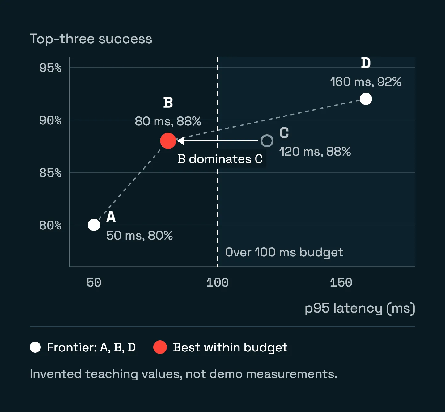
The dashed line is a visual guide between the invented configurations, not a set of measured intermediate results.
Look at B and C. They achieve the same quality, but B is faster. B dominates C: on the measures we’re comparing, C gives us no advantage.
A, B and D involve a choice. These are the options on the frontier: to get more quality from this set, we have to accept more latency. If our p95 budget is 100 ms, B gives us the highest quality that fits. Allowing 160 ms makes D an option.
We can consider cost and memory too. The point is to choose using the constraints of our application. And the quality measure needs to reflect the customer’s task: finding the nearest vectors isn’t enough if the products still don’t answer the request.
What we learned from the camera shop
We started with two customers: one who knew the model they wanted, and another who could only describe what they wanted to do. Following their searches took us through several parts of the system:
- Prepare the product information. Titles, descriptions and bullet points become searchable passages, with links back to the original products.
- Match words and meaning. Full-text search ranks matching terms; vector search finds passages through learned relationships. Hybrid combines their rankings, but our results showed why we still need to check what reaches the top.
- Judge the answer against the request. A related camera can be the wrong model, and a wildlife camera is still not the lens someone asked for. Better product fields and clearer requests can matter as much as a different ranking method.
- Keep search current. Product changes need to reach the passage records and indexes. Background workers, retries and switching between index versions all affect whether customers can find the current catalogue.
- Measure the whole wait. Query embedding, retrieval and product loading all contribute to latency. Improving results means choosing trade-offs that fit the shop’s time, memory and cost budgets.
You can try the demo code with queries you care about. Write down what would make an answer useful, then look at what comes back. Even a highly ranked result can leave you looking for the camera you wanted.
Do you have any thoughts, corrections or questions? I'd love to hear from you.
Get the next note
New notes when I publish. No schedule, no filler.